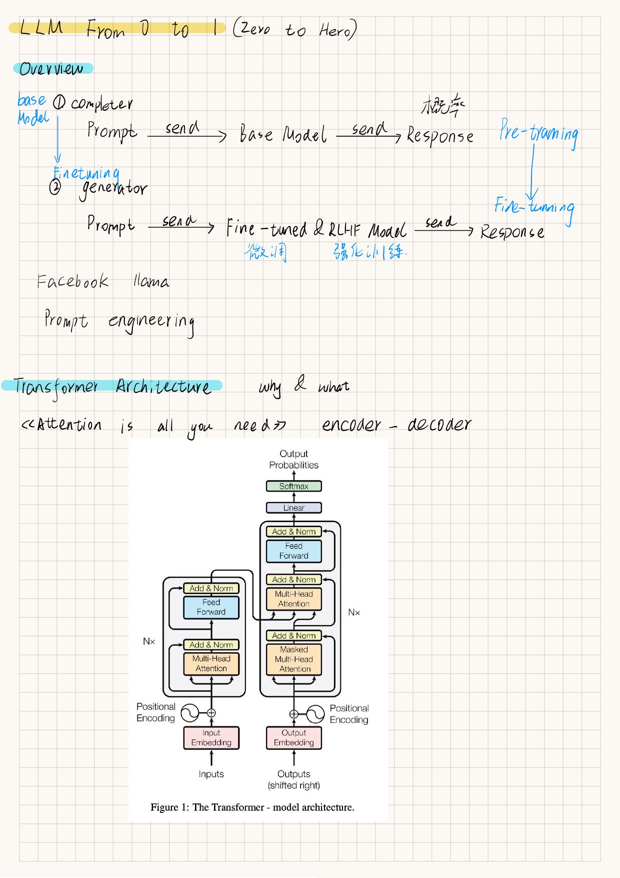
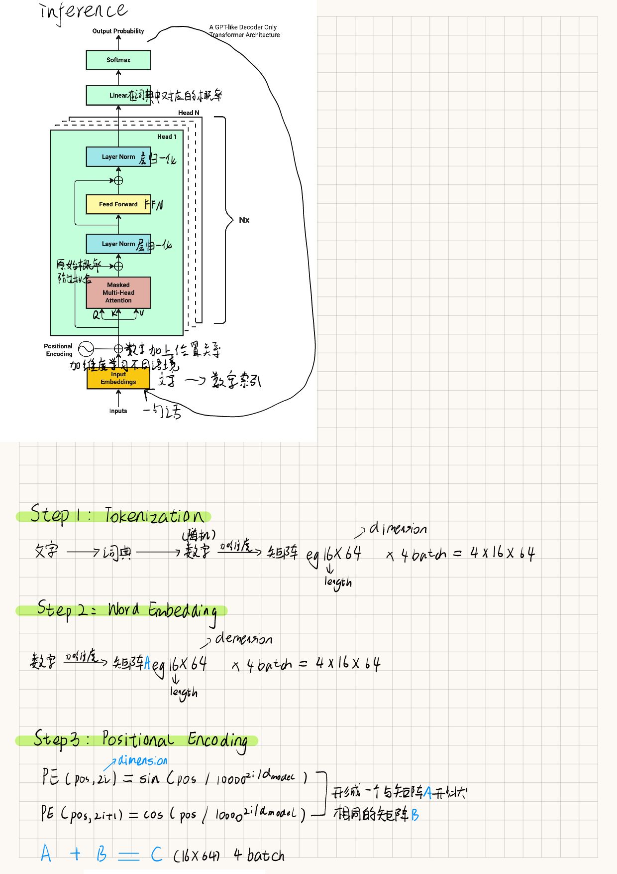
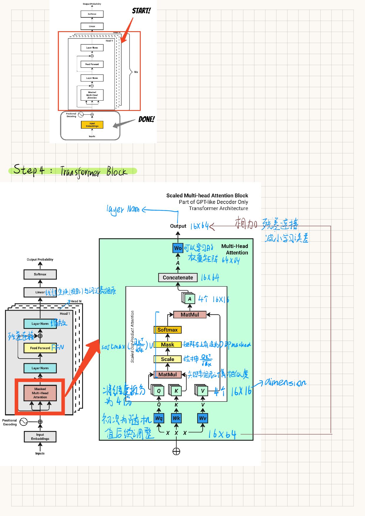
1. 1. 框架基本知识
  2. 2. 代码
  3. 3. 效果
  4. 4. Post-LayerNorm vs Pre-LayerNorm
    1. 4.1. 两种 LayerNorm 位置对比
    2. 4.2. 为什么要改为 Pre-LayerNorm?
      1. 4.2.1. 训练稳定性大幅提升
      2. 4.2.2. 收敛速度更快
      3. 4.2.3. 梯度传播更直接
    3. 4.3. 梯度计算对比
    4. 4.4. 总结
  5. 5. 改进
  6. 6. LayerNorm
    1. 6.1. 什么是层归一化?
    2. 6.2. 层归一化 vs. 批归一化(Batch Normalization)
    3. 6.3. 层归一化的主要作用
      1. 6.3.1. 稳定训练过程
      2. 6.3.2. 加速收敛
      3. 6.3.3. 减少对参数初始化的依赖
      4. 6.3.4. 轻微的正则化效果
    4. 6.4. 在 Transformer 中的典型应用
  7. 7. 微调(Fine-tuning)
    1. 7.1. 微调的原理
      1. 7.1.1. 为什么微调有效?
      2. 7.1.2. 微调的数学本质
    2. 7.2. 微调的步骤
      1. 7.2.1. 步骤1:准备任务数据集
      2. 7.2.2. 步骤2:加载预训练模型和分词器
      3. 7.2.3. 步骤3:配置微调参数
      4. 7.2.4. 步骤4:执行训练
      5. 7.2.5. 步骤5:评估与保存
      6. 7.2.6. (可选)步骤6:部署
    3. 7.3. 微调的注意事项
    4. 7.4. 常见微调类型简介
  8. 8. 线性变换
    1. 8.1. 矩阵计算
  9. 9. Decoding Strategies 推理策略
    1. 9.0.1. 贪心搜索 (Greedy Search)
    2. 9.0.2. 纯随机采样 (Random Sampling)
    3. 9.0.3. Top-K 采样 (固定数量截断)
    4. 9.0.4. Top-P 采样 (核采样 Nucleus Sampling)
    5. 9.0.5. 束搜索 (Beam Search)
    6. 9.0.6. Temperature
  • 10. 知识拾遗
    1. 10.1. Python 装饰器
      1. 10.1.1. 基本概念
    2. 10.2. 装饰器的基本用法
      1. 10.2.1. 最简单的装饰器
      2. 10.2.2. 装饰带参数的函数
    3. 10.3. 装饰器的四种形式
      1. 10.3.1. 形式1:函数装饰器(最常用)
      2. 10.3.2. 形式2:带参数的装饰器
      3. 10.3.3. 形式3:类装饰器
      4. 10.3.4. 形式4:多个装饰器堆叠
    4. 10.4. 装饰器在实际项目中的应用
      1. 10.4.1. 日志记录
      2. 10.4.2. 权限验证
      3. 10.4.3. 缓存/记忆化
      4. 10.4.4. 重试机制
    5. 10.5. 使用 functools.wraps
      1. 10.5.1. 为什么需要它?
    6. 10.6. 装饰器的底层原理
      1. 10.6.1. 装饰器的执行时机
    7. 10.7. 在机器学习中的实际应用
      1. 10.7.1. 模型训练装饰器
      2. 10.7.2. 梯度检查装饰器
    8. 10.8. 装饰器的常见问题
      1. 10.8.1. 问题1:装饰器破坏了函数签名
      2. 10.8.2. 问题2:装饰器不能装饰类方法
      3. 10.8.3. 问题3:装饰器影响性能
    9. 10.9. 装饰器的最佳实践
      1. 10.9.1. 始终使用 functools.wraps
      2. 10.9.2. 编写可重用的装饰器
      3. 10.9.3. 装饰器工厂模式
    10. 10.10. 总结
    11. 10.11. model.train() model.eval()
    12. 10.12. 广播机制(Broadcasting)
      1. 10.12.1. 广播规则
        1. 10.12.1.1. 规则1:维度对齐(从右向左)
        2. 10.12.1.2. 规则2:兼容性判断
        3. 10.12.1.3. 规则3:扩展执行
    13. 10.13. unsqueeze() squeeze()
    14. 10.14. view() reshape()
      1. 10.14.1. 其他改变形状的API
  • 从0实现Transformer

    大模型《从零到一》长视频系列

    框架基本知识

    深度学习_0

    深度学习_1

    深度学习_2

    代码

    1.实现的是解码器结构的Transformer而非原始论文的encode-decode

    2.和原始论文不太一样,并且存在许多隐含错误

    1
    2
    3
    4
    5
    6
    7
    8
    9
    10
    11
    12
    13
    14
    15
    16
    17
    18
    19
    20
    21
    22
    23
    24
    25
    26
    27
    28
    29
    30
    31
    32
    33
    34
    35
    36
    37
    38
    39
    40
    41
    42
    43
    44
    45
    46
    47
    48
    49
    50
    51
    52
    53
    54
    55
    56
    57
    58
    59
    60
    61
    62
    63
    64
    65
    66
    67
    68
    69
    70
    71
    72
    73
    74
    75
    76
    77
    78
    79
    80
    81
    82
    83
    84
    85
    86
    87
    88
    89
    90
    91
    92
    93
    94
    95
    96
    97
    98
    99
    100
    101
    102
    103
    104
    105
    106
    107
    108
    109
    110
    111
    112
    113
    114
    115
    116
    117
    118
    119
    120
    121
    122
    123
    124
    125
    126
    127
    128
    129
    130
    131
    132
    133
    134
    135
    136
    137
    138
    139
    140
    141
    142
    143
    144
    145
    146
    147
    148
    149
    150
    151
    152
    153
    154
    155
    156
    157
    158
    159
    160
    161
    162
    163
    164
    165
    166
    167
    168
    169
    170
    171
    172
    173
    174
    175
    176
    177
    178
    179
    180
    181
    182
    183
    184
    185
    186
    187
    188
    189
    190
    191
    192
    193
    194
    195
    196
    197
    198
    199
    200
    201
    202
    203
    204
    205
    206
    207
    208
    209
    210
    211
    212
    213
    214
    215
    216
    217
    218
    219
    220
    221
    222
    223
    224
    225
    226
    227
    228
    229
    230
    231
    232
    233
    234
    235
    236
    237
    238
    239
    240
    241
    242
    243
    244
    245
    246
    247
    248
    249
    250
    251
    252
    253
    254
    255
    256
    257
    258
    259
    260
    261
    262
    263
    '''
    Decoder-Only transformer
    '''


    import os
    import torch
    import torch.nn as nn
    import torch.nn.functional as F
    import requests
    import tiktoken
    import math


    # 超参数
    batch_size = 4
    context_len = 16
    d_model = 64 # 每个token的维度
    num_blocks = 8 #循环多少次
    num_heads = 4 #分为几个头
    learning_rate = 1e-3
    dropout = 0.1

    max_iters = 500#迭代多少次
    eval_interval = 50
    eval_iters = 100
    device = 'cuda' if torch.cuda.is_available() else 'cpu'
    TORCH_SEED = 1337
    torch.manual_seed(TORCH_SEED)


    # get dataset
    if not os.path.exists('/home/lizy/graduate/Transformer_learning/sales_textbook.txt'):
    url = 'https://huggingface.co/datasets/goendalf666/sales-textbook_for_convincing_and_selling/raw/main/sales_textbook.txt'
    with open('/home/lizy/graduate/Transformer_learning/sales_textbook.txt','wb') as f:
    f.write(requests.get(url).content)
    with open('/home/lizy/graduate/Transformer_learning/sales_textbook.txt','r', encoding='utf-8') as f:
    text = f.read()


    encoding = tiktoken.get_encoding("cl100k_base")
    vocab_size = encoding.n_vocab # tiktoken的词汇表大小

    tokenized_text = encoding.encode(text)
    # max_token_value = tokenized_text.max().item() + 1
    tokenized_text=torch.tensor(tokenized_text,dtype=torch.long,device=device)


    train_idex = int(len(tokenized_text) * 0.9)
    train_data = tokenized_text[:train_idex]
    valid_data = tokenized_text[train_idex:]


    class FeedforwardNetwork(nn.Module):
    def __init__(self,d_model,d_ff):
    super(FeedforwardNetwork,self).__init__()
    self.linear1 = nn.Linear(d_model,d_ff)
    self.ReLU = nn.ReLU()
    self.linear2 = nn.Linear(d_ff,d_model)
    self.dropout = nn.Dropout(dropout)

    def forward(self,x):
    x=self.linear1(x)
    x=self.ReLU(x)
    x=self.linear2(x)
    x=self.dropout(x)

    return x

    class ScaledDotProductAttention(nn.Module):
    def __init__(self):
    super().__init__()
    self.Wq = nn.Linear(d_model,d_model//num_heads)
    self.Wk = nn.Linear(d_model,d_model//num_heads)
    self.Wv = nn.Linear(d_model,d_model//num_heads)

    self.register_buffer('mask',torch.tril(torch.ones(context_len,context_len)))
    self.dropout = nn.Dropout(dropout)

    def forward(self,x):

    B, T, C = x.shape # Batch size, Time steps(current context_length), Channels(dimensions)
    assert T <= context_len
    assert C == d_model

    Q = self.Wq(x)
    K = self.Wk(x)
    V = self.Wv(x)
    #单头注意力
    attention = Q @ K.transpose(-2,-1) / math.sqrt(d_model//num_heads)
    attention = attention.masked_fill(self.mask[:T, :T] == 0, float('-inf'))
    attention = F.softmax(attention,dim=-1)
    attention = self.dropout(attention)
    return attention @ V #signal head output (B,T,head_dim)

    class MultiHeadAttention(nn.Module):
    def __init__(self):
    super().__init__()
    self.heads = nn.ModuleList([ScaledDotProductAttention() for _ in range(num_heads)]) #多头
    self.projection_layer = nn.Linear(d_model,d_model)
    self.dropout = nn.Dropout(dropout)

    def forward(self,x):
    heads_output = [head(x) for head in self.heads]
    out = torch.cat(heads_output,dim=-1)
    out = self.projection_layer(out)
    out = self.dropout(out)

    return out

    class TransformerBlock(nn.Module):
    def __init__(self):
    super().__init__()
    self.multi_head_attention_layer = MultiHeadAttention()
    self.ffn = FeedforwardNetwork(d_model,d_model*4)
    self.layer_norm_1=nn.LayerNorm(d_model)
    self.layer_norm_2=nn.LayerNorm(d_model)
    def forward(self,x):
    x = x + self.multi_head_attention_layer(x)
    x = self.layer_norm_1(x)
    x = x + self.ffn(x)
    x = self.layer_norm_2(x)

    return x

    class TransformerLanguageModel(nn.Module):
    def __init__(self):
    super().__init__()
    #self.token_embedding_lookup_table = nn.Embedding(max_token_value+1,d_model)
    # 应该使用tokenizer的实际词汇表大小
    self.token_embedding_lookup_table = nn.Embedding(vocab_size, d_model)


    self.transformer_blocks = nn.Sequential(*(
    [TransformerBlock() for _ in range(num_blocks)]
    # + [nn.LayerNorm(d_model)]#Different from original paper, here we add a final layer norm after all the blocks
    ))

    self.language_model_out_linear_layer = nn.Linear(d_model,vocab_size)

    def forward(self,idx,targets=None):
    B , T = idx.shape

    position_encoding_lookup_table = torch.zeros(context_len,d_model)
    position = torch.arange(0,context_len,dtype=torch.float).unsqueeze(1)
    div_term = torch.exp(torch.arange(0, d_model, 2).float() * (-math.log(10000.0) / d_model))
    position_encoding_lookup_table[:, 0::2] = torch.sin(position * div_term)
    position_encoding_lookup_table[:, 1::2] = torch.cos(position * div_term)

    position_embedding = position_encoding_lookup_table[:T, :].to(device)

    x = self.token_embedding_lookup_table(idx) + position_embedding
    x = self.transformer_blocks(x)

    logits = self.language_model_out_linear_layer(x)

    if targets is not None:
    B, T, C = logits.shape
    logits_reshaped = logits.view(B * T, C)
    targets_reshaped = targets.view(B * T)
    loss = F.cross_entropy(input=logits_reshaped, target=targets_reshaped)
    else:
    loss = None
    return logits, loss


    def generate(self, idx, max_new_tokens, temperature=0.8, top_k=50):
    for _ in range(max_new_tokens):
    idx_crop = idx[:, -context_len:] if idx.size(1) > context_len else idx

    logits, _ = self(idx_crop)
    logits = logits[:, -1, :] / temperature

    # 可选:top-k采样,提高质量
    if top_k is not None:
    v, _ = torch.topk(logits, min(top_k, logits.size(-1)))
    logits[logits < v[:, [-1]]] = float('-inf')

    probs = F.softmax(logits, dim=-1)

    # 采样
    idx_next = torch.multinomial(probs, num_samples=1)

    # 确保token在有效范围内
    idx_next = torch.clamp(idx_next, 0, vocab_size - 1)

    idx = torch.cat((idx, idx_next), dim=1)

    return idx


    model = TransformerLanguageModel()
    model = model.to(device)

    def get_batch(split):
    data = train_data if split == 'train' else valid_data
    idxs = torch.randint(low=0, high=len(data) - context_len, size=(batch_size,))
    x = torch.stack([data[idx:idx + context_len] for idx in idxs]).to(device)
    y = torch.stack([data[idx + 1:idx + context_len + 1] for idx in idxs]).to(device)
    return x, y


    # Calculate loss
    @torch.no_grad()
    def estimate_loss():
    out = {}
    model.eval() # 用于将模型设置为评估模式
    for split in ['train', 'valid']:
    losses = torch.zeros(eval_iters)
    for k in range(eval_iters):
    x_batch, y_batch = get_batch(split)
    logits, loss = model(x_batch, y_batch)
    losses[k] = loss.item()
    out[split] = losses.mean()
    model.train()
    return out

    # 训练
    optimizer = torch.optim.AdamW(params=model.parameters(), lr=learning_rate)
    tracked_losses = list()
    for step in range(max_iters):
    if step % eval_iters == 0 or step == max_iters - 1:
    losses = estimate_loss()
    tracked_losses.append(losses)
    print('Step:', step, 'Training Loss:', round(losses['train'].item(), 3), 'Validation Loss:',
    round(losses['valid'].item(), 3))

    xb, yb = get_batch('train')
    logits, loss = model(xb, yb)
    optimizer.zero_grad(set_to_none=True)
    loss.backward()
    optimizer.step()

    # Save the model state dictionary
    torch.save(model.state_dict(), 'model-ckpt.pt')


    # Generate
    model.eval()
    start = 'The salesperson'
    start_ids = encoding.encode(start)
    x = (torch.tensor(start_ids, dtype=torch.long, device=device)[None, ...])
    y = model.generate(x, max_new_tokens=100)
    print('---------------')
    #
    try:
    generated_text = encoding.decode(y[0].tolist())
    except KeyError as e:
    print(f"解码时遇到无效token,尝试忽略: {e}")
    # 忽略无效token
    valid_tokens = []
    for token in y[0].tolist():
    try:
    # 检查token是否有效
    if 0 <= token < vocab_size:
    valid_tokens.append(token)
    except:
    continue
    generated_text = encoding.decode(valid_tokens)

    print(encoding.decode(y[0].tolist()))
    print('---------------')

    效果

    1
    2
    3
    4
    5
    6
    7
    8
    9
    10
    11
    12
    13
    14
    15
    16
    17
    18
    19
    20
    21
    22
    23
    24
    25
    26
    27
    28
    29
    30
    31
    32
    33
    34
    35
    36
    37
    38
    39
    40
    41
    42
    43
    44
    45
    46
    47
    48
    49
    50
    51
    52
    53
    54
    Step: 0 Training Loss: 11.705 Validation Loss: 11.714
    Step: 100 Training Loss: 6.766 Validation Loss: 7.352
    Step: 200 Training Loss: 6.263 Validation Loss: 6.846
    Step: 300 Training Loss: 5.778 Validation Loss: 6.467
    Step: 400 Training Loss: 5.465 Validation Loss: 6.212
    Step: 500 Training Loss: 5.272 Validation Loss: 6.144
    Step: 600 Training Loss: 4.886 Validation Loss: 5.937
    Step: 700 Training Loss: 4.84 Validation Loss: 5.865
    Step: 800 Training Loss: 4.691 Validation Loss: 5.746
    Step: 900 Training Loss: 4.508 Validation Loss: 5.787
    Step: 1000 Training Loss: 4.504 Validation Loss: 5.763
    Step: 1100 Training Loss: 4.412 Validation Loss: 5.549
    Step: 1200 Training Loss: 4.237 Validation Loss: 5.498
    Step: 1300 Training Loss: 4.289 Validation Loss: 5.356
    Step: 1400 Training Loss: 4.156 Validation Loss: 5.582
    Step: 1500 Training Loss: 4.024 Validation Loss: 5.308
    Step: 1600 Training Loss: 4.047 Validation Loss: 5.403
    Step: 1700 Training Loss: 3.915 Validation Loss: 5.366
    Step: 1800 Training Loss: 3.909 Validation Loss: 5.254
    Step: 1900 Training Loss: 3.917 Validation Loss: 5.205
    Step: 2000 Training Loss: 3.836 Validation Loss: 5.26
    Step: 2100 Training Loss: 3.771 Validation Loss: 5.132
    Step: 2200 Training Loss: 3.793 Validation Loss: 5.269
    Step: 2300 Training Loss: 3.579 Validation Loss: 5.268
    Step: 2400 Training Loss: 3.661 Validation Loss: 5.207
    Step: 2500 Training Loss: 3.625 Validation Loss: 5.102
    Step: 2600 Training Loss: 3.6 Validation Loss: 4.921
    Step: 2700 Training Loss: 3.502 Validation Loss: 5.028
    Step: 2800 Training Loss: 3.503 Validation Loss: 4.943
    Step: 2900 Training Loss: 3.437 Validation Loss: 4.943
    Step: 3000 Training Loss: 3.441 Validation Loss: 4.992
    Step: 3100 Training Loss: 3.348 Validation Loss: 4.964
    Step: 3200 Training Loss: 3.338 Validation Loss: 4.93
    Step: 3300 Training Loss: 3.377 Validation Loss: 5.002
    Step: 3400 Training Loss: 3.205 Validation Loss: 4.944
    Step: 3500 Training Loss: 3.353 Validation Loss: 4.872
    Step: 3600 Training Loss: 3.279 Validation Loss: 4.988
    Step: 3700 Training Loss: 3.267 Validation Loss: 5.028
    Step: 3800 Training Loss: 3.307 Validation Loss: 4.805
    Step: 3900 Training Loss: 3.184 Validation Loss: 4.879
    Step: 4000 Training Loss: 3.231 Validation Loss: 4.911
    Step: 4100 Training Loss: 3.128 Validation Loss: 4.968
    Step: 4200 Training Loss: 3.089 Validation Loss: 4.928
    Step: 4300 Training Loss: 3.092 Validation Loss: 4.938
    Step: 4400 Training Loss: 3.136 Validation Loss: 4.978
    Step: 4500 Training Loss: 3.047 Validation Loss: 4.791
    Step: 4600 Training Loss: 2.983 Validation Loss: 4.931
    Step: 4700 Training Loss: 3.052 Validation Loss: 4.975
    Step: 4800 Training Loss: 3.027 Validation Loss: 4.828
    Step: 4900 Training Loss: 3.001 Validation Loss: 4.792
    Step: 4999 Training Loss: 2.933 Validation Loss: 4.921
    ---------------
    The salesperson should create a connection with potential customer that your customers, ensuring the customer with your customers, and avoiding jargon. By actively listening, you can establish a solidify and build trust. For example, you can build trust, and credibility, credibility, build credibility and credibility, as them to make a more favorable, you can effectively communicate your unique circumstances, take action promptly to the customer's perspective and understanding. By utilizing the ideal solution that your product or service limitations, you can build trust and increase
    ---------------

    Post-LayerNorm vs Pre-LayerNorm

    后来的 Transformer 模型普遍从原始的 Post-LayerNorm 改为 Pre-LayerNorm

    两种 LayerNorm 位置对比

    原始 Transformer(Post-LayerNorm)

    1
    2
    3
    # 原始论文的顺序:子层 → LayerNorm → 残差连接
    x = x + Sublayer(x) # 先计算子层输出
    x = LayerNorm(x) # 再归一化

    现代 Transformer(Pre-LayerNorm)

    1
    2
    3
    # 现代实现的顺序:LayerNorm → 子层 → 残差连接
    x_norm = LayerNorm(x) # 先归一化
    x = x + Sublayer(x_norm) # 再计算子层并残差连接

    为什么要改为 Pre-LayerNorm?

    训练稳定性大幅提升

    Post-LayerNorm 的问题:

    1
    2
    3
    4
    5
    6
    # 梯度流经的路径:
    损失 → 层归一化 → 子层 → 输入
    # 梯度必须先通过层归一化,这可能导致:
    # 1. 梯度消失/爆炸(尤其深层网络)
    # 2. 需要精细的初始化
    # 3. 学习率需要小心调整

    Pre-LayerNorm 的优势:

    1
    2
    3
    4
    # 梯度流经的路径:
    损失 → 子层 → 层归一化 → 输入
    # 梯度直接通过子层,然后才到归一化
    # 梯度流动更平滑,训练更稳定

    收敛速度更快

    实际效果对比:

    • Post-LayerNorm:可能需要更多训练步数才能收敛
    • Pre-LayerNorm:通常收敛更快,需要的训练步数更少

    梯度传播更直接

    1
    2
    3
    4
    5
    6
    7
    8
    9
    10
    11
    Post-LayerNorm 梯度路径:
    损失 → LN → Attention/FFN → 输入

    梯度先经过LN的缩放操作
    可能放大或缩小梯度值

    Pre-LayerNorm 梯度路径:
    损失 → Attention/FFN → LN → 输入

    梯度直接传到子层
    LN只影响前向传播,不影响梯度回传

    梯度计算对比

    Post-LayerNorm(层归一化在残差连接后)

    1
    x = LayerNorm(x + Sublayer(x))

    反向传播的路径:

    1
    2
    3
    4
    5
    6
    7
    8
    9
    10
    11
    12
    13
    14
    梯度流向:损失 → LayerNorm → (残差连接 + Sublayer) → 输入

    梯度必须先通过LayerNorm
    它的导数可能放大或缩小梯度

    # 数学理解
    设:y = LN(x + f(x)),其中LN是LayerNorm

    梯度:∂L/∂x = ∂L/∂y × ∂LN/∂(x+f(x)) × (1 + ∂f/∂x)

    注意:∂LN/∂(x+f(x)) 包含:
    1. 1/σ 缩放(标准差倒数)
    2. 减去均值的影响
    3. gamma参数的缩放
    • 当输入x+f(x)的方差σ很小时,1/σ很大 做完乘积→ 梯度爆炸
    • 当方差σ很大时,1/σ很小 做完乘积→ 梯度消失

    Pre-LayerNorm(层归一化在残差连接前)

    1
    x = x + Sublayer(LayerNorm(x))

    反向传播的路径:

    1
    2
    3
    4
    5
    6
    7
    8
    9
    10
    11
    12
    13
    14
    15
    梯度流向:损失 → (残差连接 + Sublayer) → LayerNorm → 输入

    梯度有两条路径:
    1. 直接通过残差连接(稳定)
    2. 通过Sublayer和LayerNorm(可能变化)

    # 数学理解
    Pre-LayerNorm: y = x + f(LN(x))

    ∂L/∂x = ∂L/∂y × (∂y/∂x)
    = ∂L/∂y × [1 + ∂f/∂LN(x) × ∂LN/∂x]

    # 注意这里的 "1" 来自残差连接
    # 即使 ∂f/∂LN(x) × ∂LN/∂x 很小,
    # 仍然有 ∂L/∂y × 1 这部分梯度直接传回

    使用 Pre-LayerNorm 的模型

    1. GPT 系列(GPT-2, GPT-3, GPT-4)
    2. BERT 及其变体
    3. T5
    4. RoBERTa
    5. ALBERT
    6. 大部分现代 Transformer 变体

    使用 Post-LayerNorm 的模型

    1. 原始 Transformer(2017)
    2. 早期实验性模型
    3. 现在基本不再使用

    总结

    从 Post-LayerNorm 改为 Pre-LayerNorm 的主要原因:

    1. 训练稳定性:Pre-LayerNorm 大大减少了梯度问题
    2. 收敛速度:训练更快,需要更少的迭代次数
    3. 调参友好:对初始化和学习率不那么敏感
    4. 扩展性:更容易训练深层和超大模型
    5. 实际效果:在几乎所有任务上都表现更好

    改进

    1. 将post-LayerNorm改为pre-LayerNorm
    2. 由于原始论文中位置编码固定,因此改变位置编码的位置,避免重复计算位置编码
    3. 修改ScaledDotProductAttention类和MultiHeadAttention类的职责分配,合成一个类
    4. 在残差连接前增加Dropout层
    1
    2
    3
    4
    5
    6
    7
    8
    9
    10
    11
    12
    13
    14
    15
    16
    17
    18
    19
    20
    21
    22
    23
    24
    25
    26
    27
    28
    29
    30
    31
    32
    33
    34
    35
    36
    37
    38
    39
    40
    41
    42
    43
    44
    45
    46
    47
    48
    49
    50
    51
    52
    53
    54
    55
    56
    57
    58
    59
    60
    61
    62
    63
    64
    65
    66
    67
    68
    69
    70
    71
    72
    73
    74
    75
    76
    77
    78
    79
    80
    81
    82
    83
    84
    85
    86
    87
    88
    89
    90
    91
    92
    93
    94
    95
    96
    97
    98
    99
    100
    101
    102
    103
    104
    105
    106
    107
    108
    109
    110
    111
    112
    113
    114
    115
    116
    117
    118
    119
    120
    121
    122
    123
    124
    125
    126
    127
    128
    129
    130
    131
    132
    133
    134
    135
    136
    137
    138
    139
    140
    141
    142
    143
    144
    145
    146
    147
    148
    149
    150
    151
    152
    153
    154
    155
    156
    157
    158
    159
    160
    161
    162
    163
    164
    165
    166
    167
    168
    169
    170
    171
    172
    173
    174
    175
    176
    177
    178
    179
    180
    181
    182
    183
    184
    185
    186
    187
    188
    189
    190
    191
    192
    193
    194
    195
    196
    197
    198
    199
    200
    201
    202
    203
    204
    205
    206
    207
    208
    209
    210
    211
    212
    213
    214
    215
    216
    217
    218
    219
    220
    221
    222
    223
    224
    225
    226
    227
    228
    229
    230
    231
    232
    233
    234
    235
    236
    237
    238
    239
    240
    241
    242
    243
    244
    245
    246
    247
    248
    249
    250
    251
    252
    253
    '''
    Decoder-Only transformer

    pre layerNorm
    '''

    import os
    import torch
    import torch.nn as nn
    import torch.nn.functional as F
    import requests
    import tiktoken
    import math


    # 超参数
    batch_size = 4
    context_len = 16
    d_model = 64 # 每个token的维度
    num_blocks = 8 #循环多少次
    num_heads = 4 #分为几个头
    learning_rate = 1e-3
    dropout = 0.1

    max_iters = 5000 # 一共迭代多少次
    eval_interval = 100 # 多久评估一次
    eval_iters = 100 # 评估时的计算轮次
    device = 'cuda' if torch.cuda.is_available() else 'cpu'
    TORCH_SEED = 1337
    torch.manual_seed(TORCH_SEED)


    # get dataset
    if not os.path.exists('/home/lizy/graduate/Transformer_learning/sales_textbook.txt'):
    url = 'https://huggingface.co/datasets/goendalf666/sales-textbook_for_convincing_and_selling/raw/main/sales_textbook.txt'
    with open('/home/lizy/graduate/Transformer_learning/sales_textbook.txt','wb') as f:
    f.write(requests.get(url).content)
    with open('/home/lizy/graduate/Transformer_learning/sales_textbook.txt','r', encoding='utf-8') as f:
    text = f.read()


    encoding = tiktoken.get_encoding("cl100k_base")
    vocab_size = encoding.n_vocab # tiktoken的词汇表大小

    tokenized_text = encoding.encode(text)
    # max_token_value = tokenized_text.max().item() + 1
    tokenized_text=torch.tensor(tokenized_text,dtype=torch.long,device=device)


    train_idex = int(len(tokenized_text) * 0.9)
    train_data = tokenized_text[:train_idex]
    valid_data = tokenized_text[train_idex:]


    class FeedforwardNetwork(nn.Module):
    def __init__(self,d_model,d_ff):
    super(FeedforwardNetwork,self).__init__()
    self.linear1 = nn.Linear(d_model,d_ff)
    self.ReLU = nn.ReLU()
    self.linear2 = nn.Linear(d_ff,d_model)
    self.dropout = nn.Dropout(dropout)

    def forward(self,x):
    x=self.linear1(x)
    x=self.ReLU(x)
    x=self.linear2(x)
    x=self.dropout(x)

    return x


    class MultiHeadAttention(nn.Module):
    def __init__(self):
    super().__init__()
    self.Wqkv = nn.Linear(d_model,d_model*3) #一次计算Q K V
    self.projection_layer = nn.Linear(d_model,d_model)
    self.dropout = nn.Dropout(dropout)

    def forward(self,x):
    B,T,C = x.shape
    #一次计算所有头的QKV
    qkv = self.Wqkv(x).reshape(B,T,3,num_heads,C // num_heads)
    q,k,v = qkv.unbind(dim=2) # (B,T,num_heads,head_dim)
    q, k, v = q.transpose(1, 2), k.transpose(1, 2), v.transpose(1, 2) # (B,num_heads,T,head_dim)

    # 注意力计算
    attn = (q @ k.transpose(-2, -1)) / math.sqrt(C // num_heads) #(B, num_heads, T, T)
    mask = torch.tril(torch.ones(T, T)).to(x.device)
    attn = attn.masked_fill(mask == 0, float('-inf'))
    attn = F.softmax(attn, dim=-1)
    attn = self.dropout(attn)


    out = (attn @ v).transpose(1, 2).contiguous().view(B, T, C)
    return self.projection_layer(out)

    class TransformerBlock(nn.Module):
    def __init__(self):
    super().__init__()
    self.multi_head_attention_layer = MultiHeadAttention()
    self.ffn = FeedforwardNetwork(d_model,d_model*4)
    self.layer_norm_1=nn.LayerNorm(d_model)
    self.layer_norm_2=nn.LayerNorm(d_model)

    self.dropout = nn.Dropout(dropout)
    def forward(self,x):
    x = x + self.dropout(self.multi_head_attention_layer(self.layer_norm_1(x)))
    x = x + self.dropout(self.ffn(self.layer_norm_2(x)))
    return x

    class TransformerLanguageModel(nn.Module):
    def __init__(self):
    super().__init__()
    #self.token_embedding_lookup_table = nn.Embedding(max_token_value+1,d_model)
    # 应该使用tokenizer的实际词汇表大小
    self.token_embedding_lookup_table = nn.Embedding(vocab_size, d_model)


    self.transformer_blocks = nn.Sequential(*(
    [TransformerBlock() for _ in range(num_blocks)]
    + [nn.LayerNorm(d_model)]#Different from original paper, here we add a final layer norm after all the blocks
    ))

    self.language_model_out_linear_layer = nn.Linear(d_model,vocab_size)

    #预先计算位置编码
    self.register_buffer('position_embedding', self._create_position_embedding())

    def _create_position_embedding(self):

    position_encoding_lookup_table = torch.zeros(context_len,d_model)
    position = torch.arange(0,context_len,dtype=torch.float).unsqueeze(1)
    div_term = torch.exp(torch.arange(0, d_model, 2).float() * (-math.log(10000.0) / d_model))
    position_encoding_lookup_table[:, 0::2] = torch.sin(position * div_term)
    position_encoding_lookup_table[:, 1::2] = torch.cos(position * div_term)

    return position_encoding_lookup_table

    def forward(self,idx,targets=None):
    B , T = idx.shape
    position_embedding = self.position_embedding[:T, :].to(device)

    x = self.token_embedding_lookup_table(idx) + position_embedding
    x = self.transformer_blocks(x)

    logits = self.language_model_out_linear_layer(x)

    if targets is not None:
    B, T, C = logits.shape
    logits_reshaped = logits.view(B * T, C)
    targets_reshaped = targets.view(B * T)
    loss = F.cross_entropy(input=logits_reshaped, target=targets_reshaped)
    else:
    loss = None
    return logits, loss


    def generate(self, idx, max_new_tokens, temperature=0.8, top_k=50):
    for _ in range(max_new_tokens):
    idx_crop = idx[:, -context_len:] if idx.size(1) > context_len else idx

    logits, _ = self(idx_crop)
    logits = logits[:, -1, :] / temperature

    # 可选:top-k采样,提高质量
    if top_k is not None:
    v, _ = torch.topk(logits, min(top_k, logits.size(-1)))
    logits[logits < v[:, [-1]]] = float('-inf')

    probs = F.softmax(logits, dim=-1)

    # 采样
    idx_next = torch.multinomial(probs, num_samples=1)

    # 确保token在有效范围内
    idx_next = torch.clamp(idx_next, 0, vocab_size - 1)

    idx = torch.cat((idx, idx_next), dim=1)

    return idx


    model = TransformerLanguageModel()
    model = model.to(device)

    def get_batch(split):
    data = train_data if split == 'train' else valid_data
    idxs = torch.randint(low=0, high=len(data) - context_len, size=(batch_size,))
    x = torch.stack([data[idx:idx + context_len] for idx in idxs]).to(device)
    y = torch.stack([data[idx + 1:idx + context_len + 1] for idx in idxs]).to(device)
    return x, y


    # Calculate loss
    @torch.no_grad()
    def estimate_loss():
    out = {}
    model.eval() # 用于将模型设置为评估模式
    for split in ['train', 'valid']:
    losses = torch.zeros(eval_iters)
    for k in range(eval_iters):
    x_batch, y_batch = get_batch(split)
    logits, loss = model(x_batch, y_batch)
    losses[k] = loss.item()
    out[split] = losses.mean()
    model.train()
    return out

    # 训练
    optimizer = torch.optim.AdamW(params=model.parameters(), lr=learning_rate)
    tracked_losses = list()
    for step in range(max_iters):
    if step % eval_interval == 0 or step == max_iters - 1:
    losses = estimate_loss()
    tracked_losses.append(losses)
    print('Step:', step, 'Training Loss:', round(losses['train'].item(), 3), 'Validation Loss:',
    round(losses['valid'].item(), 3))

    xb, yb = get_batch('train')
    logits, loss = model(xb, yb)
    optimizer.zero_grad(set_to_none=True)
    loss.backward()
    optimizer.step()

    # Save the model state dictionary
    torch.save(model.state_dict(), './model_para/model_pre-ckpt.pt')


    # Generate
    model.eval()
    start = 'The salesperson'
    start_ids = encoding.encode(start)
    x = (torch.tensor(start_ids, dtype=torch.long, device=device)[None, ...])
    y = model.generate(x, max_new_tokens=100)
    print('---------------')
    #
    try:
    generated_text = encoding.decode(y[0].tolist())
    except KeyError as e:
    print(f"解码时遇到无效token,尝试忽略: {e}")
    # 忽略无效token
    valid_tokens = []
    for token in y[0].tolist():
    try:
    # 检查token是否有效
    if 0 <= token < vocab_size:
    valid_tokens.append(token)
    except:
    continue
    generated_text = encoding.decode(valid_tokens)

    print(encoding.decode(y[0].tolist()))
    print('---------------')
    1
    2
    3
    4
    5
    6
    7
    8
    9
    10
    11
    12
    13
    14
    15
    16
    17
    18
    19
    20
    21
    22
    23
    24
    25
    26
    27
    28
    29
    30
    31
    32
    33
    34
    35
    36
    37
    38
    39
    40
    41
    42
    43
    44
    45
    46
    47
    48
    49
    50
    51
    52
    53
    54
    Step: 0 Training Loss: 11.68 Validation Loss: 11.693
    Step: 100 Training Loss: 6.739 Validation Loss: 7.328
    Step: 200 Training Loss: 6.219 Validation Loss: 6.781
    Step: 300 Training Loss: 5.725 Validation Loss: 6.413
    Step: 400 Training Loss: 5.387 Validation Loss: 6.186
    Step: 500 Training Loss: 5.22 Validation Loss: 6.108
    Step: 600 Training Loss: 4.842 Validation Loss: 5.907
    Step: 700 Training Loss: 4.76 Validation Loss: 5.817
    Step: 800 Training Loss: 4.651 Validation Loss: 5.722
    Step: 900 Training Loss: 4.466 Validation Loss: 5.766
    Step: 1000 Training Loss: 4.43 Validation Loss: 5.714
    Step: 1100 Training Loss: 4.353 Validation Loss: 5.496
    Step: 1200 Training Loss: 4.167 Validation Loss: 5.446
    Step: 1300 Training Loss: 4.227 Validation Loss: 5.336
    Step: 1400 Training Loss: 4.104 Validation Loss: 5.546
    Step: 1500 Training Loss: 3.981 Validation Loss: 5.33
    Step: 1600 Training Loss: 4.005 Validation Loss: 5.393
    Step: 1700 Training Loss: 3.869 Validation Loss: 5.364
    Step: 1800 Training Loss: 3.841 Validation Loss: 5.181
    Step: 1900 Training Loss: 3.87 Validation Loss: 5.169
    Step: 2000 Training Loss: 3.775 Validation Loss: 5.235
    Step: 2100 Training Loss: 3.738 Validation Loss: 5.118
    Step: 2200 Training Loss: 3.74 Validation Loss: 5.214
    Step: 2300 Training Loss: 3.522 Validation Loss: 5.215
    Step: 2400 Training Loss: 3.599 Validation Loss: 5.164
    Step: 2500 Training Loss: 3.573 Validation Loss: 5.105
    Step: 2600 Training Loss: 3.564 Validation Loss: 4.887
    Step: 2700 Training Loss: 3.45 Validation Loss: 5.05
    Step: 2800 Training Loss: 3.435 Validation Loss: 4.914
    Step: 2900 Training Loss: 3.374 Validation Loss: 4.98
    Step: 3000 Training Loss: 3.387 Validation Loss: 4.99
    Step: 3100 Training Loss: 3.292 Validation Loss: 4.934
    Step: 3200 Training Loss: 3.263 Validation Loss: 4.946
    Step: 3300 Training Loss: 3.309 Validation Loss: 5.0
    Step: 3400 Training Loss: 3.15 Validation Loss: 4.967
    Step: 3500 Training Loss: 3.27 Validation Loss: 4.829
    Step: 3600 Training Loss: 3.241 Validation Loss: 4.995
    Step: 3700 Training Loss: 3.195 Validation Loss: 5.018
    Step: 3800 Training Loss: 3.251 Validation Loss: 4.801
    Step: 3900 Training Loss: 3.132 Validation Loss: 4.875
    Step: 4000 Training Loss: 3.157 Validation Loss: 4.883
    Step: 4100 Training Loss: 3.062 Validation Loss: 4.917
    Step: 4200 Training Loss: 3.007 Validation Loss: 4.918
    Step: 4300 Training Loss: 3.032 Validation Loss: 4.943
    Step: 4400 Training Loss: 3.075 Validation Loss: 4.97
    Step: 4500 Training Loss: 2.999 Validation Loss: 4.808
    Step: 4600 Training Loss: 2.899 Validation Loss: 4.985
    Step: 4700 Training Loss: 2.993 Validation Loss: 4.971
    Step: 4800 Training Loss: 2.942 Validation Loss: 4.867
    Step: 4900 Training Loss: 2.941 Validation Loss: 4.835
    Step: 4999 Training Loss: 2.871 Validation Loss: 4.932
    ---------------
    The salesperson can create a more likely in price and concise explanations. By asking follow-up questions, you create an environment where and clarifying their pain points. By showcasing the art of closing the sales process, such as the, and commitment to address their pain points, you offer tailored information or modifications to potential customers. By recognizing the time to product or service, salespeople can establish them see the sense of urgency and persuasion. This technique of clarifying the customer's responses, further reinforce the price or budget.
    ---------------

    可能是有点提升,但我不知道是哪个发挥了作用

    LayerNorm

    层归一化(Layer Normalization) 是一种广泛应用于深度学习模型(尤其是 Transformer 架构)的归一化技术。它的核心思想是对单个样本的所有特征维度进行归一化,使得每一层的输出具有稳定的分布,从而加速训练并提高模型性能。


    什么是层归一化?

    对于一个输入向量$ ( x \in \mathbb{R}^d )($即单个样本的 $ d $个特征,层归一化计算该样本自身的均值和方差:

    $
    \mu = \frac{1}{d} \sum_{i=1}^{d} x_i, \quad \sigma^2 = \frac{1}{d} \sum_{i=1}^{d} (x_i - \mu)^2
    $

    然后对每个特征进行归一化:

    $
    \hat{x}_i = \frac{x_i - \mu}{\sqrt{\sigma^2 + \epsilon}}
    $

    这里的 $\epsilon$是一个很小的常数,防止除零。

    最后引入可学习的缩放参数 ($\gamma$) 和平移参数 ($\beta$)(与输入维度相同),恢复模型的表达能力:

    $
    y_i = \gamma_i \hat{x}_i + \beta_i
    $


    层归一化 vs. 批归一化(Batch Normalization)

    特性 批归一化 (BN) 层归一化 (LN)
    归一化维度 在 batch 维度上,对每个特征通道归一化 在特征维度上,对每个样本归一化
    依赖 batch size 依赖 batch 大小,小 batch 效果差 不依赖 batch 大小,单样本也可用
    适用场景 CNN 等固定尺寸输入 RNN、Transformer 等变长序列
    训练与测试差异 训练时使用 batch 统计量,测试时使用全局移动平均 训练和测试行为一致,均使用当前样本统计量

    为什么 Transformer 偏爱层归一化?
    因为 Transformer 处理的是变长的序列,且在不同任务中 batch size 可能很小,使用批归一化会导致统计量不稳定;而层归一化对每个样本独立计算,天然适用于变长输入,且实现简单、稳定。


    层归一化的主要作用

    稳定训练过程

    • 缓解梯度消失/爆炸:归一化将输入拉回到一个合适的范围,使得反向传播的梯度不会过大或过小,从而避免梯度问题。
    • 平滑损失曲面:使损失函数对参数的变化更不敏感,优化路径更平滑,训练更稳定。

    加速收敛

    • 归一化后的输出均值为 0、方差为 1,使得后续层的输入分布相对固定,允许使用更大的学习率,从而加快模型收敛速度。

    减少对参数初始化的依赖

    • 在没有归一化的情况下,模型对权重初始化非常敏感;层归一化降低了这种敏感性,使训练更鲁棒。

    轻微的正则化效果

    • 由于每个样本的归一化引入了少量噪声(因为统计量来自当前样本),有时可以起到类似 Dropout 的正则化作用,提高泛化能力。

    在 Transformer 中的典型应用

    Transformer 的每个子层(如多头自注意力、前馈神经网络)之后都包含一个残差连接和一个层归一化,通常有两种放置方式:

    • Post-LN(原始 Transformer)LayerNorm(x + Sublayer(x))
    • Pre-LN(更常见于现代实现)x + Sublayer(LayerNorm(x))

    Pre-LN 的梯度流动更顺畅,训练更稳定,因此被 GPT、BERT 等主流模型广泛采用。


    微调(Fine-tuning)

    微调(Fine-tuning) 是深度学习和自然语言处理中非常核心的技术,尤其在预训练大模型时代,它让通用模型能够快速适配特定任务。


    微调的原理

    微调基于迁移学习的思想:一个在大规模、多样化数据上预训练好的模型,已经学习到了通用的特征表示和语言知识。我们只需要在目标任务的小规模数据集上对它进行“微小的调整”,就能让它适应新任务,而无需从头训练。

    为什么微调有效?

    • 知识复用:预训练模型(如BERT、GPT)在海量文本上学习到了语法、语义、上下文关系等通用知识。这些知识对绝大多数下游任务都有用。
    • 良好的初始化:预训练模型提供了一个比随机初始化更好的起点,使得优化过程更快、更稳定,且不容易陷入差的局部最优。
    • 数据效率高:目标任务通常只有少量标注数据,从头训练容易过拟合。微调利用预训练知识,相当于给模型一个强先验,只需少量数据就能学到任务特定的模式。

    微调的数学本质

    假设预训练模型的参数为$ \theta_{\text{pre}}$,目标任务损失函数为 $\mathcal{L}{\text{task}}$。微调的过程就是寻找一组参数 $\theta$,使得在目标任务上损失最小,同时希望 $\theta$不要偏离$ \theta{\text{pre}}$太远(防止灾难性遗忘)。因此,微调通常采用较低的初始学习率,并在少量迭代后收敛。

    对于大语言模型,微调常分为:

    • 全参数微调:更新所有预训练参数。
    • 参数高效微调:只更新少量新增参数(如LoRA、Adapter、Prefix Tuning),冻结大部分预训练参数,以降低显存消耗和避免过拟合。

    微调的步骤

    微调的一般流程包括数据准备、模型加载、训练配置、执行训练和评估。下面以有监督微调(Supervised Fine-tuning)为例说明,指令微调(Instruction Tuning)本质类似,只是数据格式变为指令-回答对。

    步骤1:准备任务数据集

    • 收集数据:根据目标任务(如情感分类、文本摘要、对话生成)收集标注数据。
    • 数据清洗:去除噪声、处理缺失值、统一格式。
    • 划分数据集:通常分为训练集、验证集和测试集(如 80%:10%:10%)。
    • 格式化:对于大语言模型,需要将数据组织成模型期望的格式。例如,对于分类任务,可构造为 [CLS] 句子 [SEP];对于生成任务,可构造为 输入:[指令] 输出:[回答]

    步骤2:加载预训练模型和分词器

    • 选择基础模型(如 LLaMA、ChatGLM、BERT),使用相应的库(HuggingFace Transformers)加载模型和分词器。
    • 如果需要参数高效微调,还需准备对应的模块(如 LoRA 的配置)。

    步骤3:配置微调参数

    • 训练参数
      • 学习率:通常比从头训练小很多,例如 1e-5 ~ 5e-5。
      • 批次大小(batch size):根据显存调整。
      • 训练轮数(epochs):通常较少(1~5轮),避免过拟合。
      • 优化器:常用 AdamW。
      • 学习率调度器:线性衰减或余弦衰减。
    • 是否冻结部分层:如果数据量少,可以只微调最后几层,冻结底层通用特征层。
    • 参数高效微调配置(如果使用):如 LoRA 的秩、目标模块等。

    步骤4:执行训练

    • 将训练数据按批次喂给模型。
    • 前向传播计算损失(如交叉熵损失)。
    • 反向传播更新参数(如果是全参数微调,更新全部参数;如果是参数高效微调,只更新新增参数)。
    • 每个 epoch 后在验证集上评估性能,防止过拟合,可保存最佳模型。

    步骤5:评估与保存

    • 在测试集上评估最终模型,使用任务相关指标(如准确率、BLEU、ROUGE)。
    • 保存模型权重和配置文件,以便后续推理部署。

    (可选)步骤6:部署

    • 将微调后的模型集成到应用系统中,提供服务。

    微调的注意事项

    • 灾难性遗忘:微调过程中可能丢失部分通用知识,尤其是在小数据集上全参数微调。可通过混合预训练任务或使用参数高效微调缓解。
    • 过拟合:由于目标任务数据量小,需使用早停、权重衰减等正则化技术。
    • 计算资源:全参数微调大模型需要较多显存(如数十GB),可使用梯度累积、混合精度训练、DeepSpeed 等技术优化。
    • 数据质量:微调效果高度依赖于标注数据的质量和多样性。

    常见微调类型简介

    类型 特点 适用场景
    全参数微调 更新所有参数,表达能力强,但资源消耗大 数据量大、任务与预训练差异大
    LoRA 在 Transformer 层添加低秩矩阵,只训练这些矩阵 资源有限、快速适配
    Adapter 插入小型适配模块,训练时只更新适配器 多任务学习、模块化
    Prefix Tuning 在输入前添加可训练的连续向量 生成任务、少样本场景
    Prompt Tuning 类似 Prefix,但只添加输入层的前缀 极轻量级微调

    参考视频:大模型《从一到N》进阶概念系列

    线性变换

    矩阵计算

    通过改变基向量来改变向量。

    对于任意输入向量 $\mathbf{v} = \begin{bmatrix} x \ y \end{bmatrix}$,由于线性变换的性质,变换后的向量等于变换后的基向量按原比例相加:

    $$
    T(\mathbf{v}) = x \cdot (\text{变换后的} \hat{i}) + y \cdot (\text{变换后的} \hat{j})
    $$

    代入坐标:

    $$
    T(\mathbf{v}) = x \begin{bmatrix} a \ b \end{bmatrix} + y \begin{bmatrix} c \ d \end{bmatrix}
    $$

    将其展开:

    $$
    T(\mathbf{v}) = \begin{bmatrix} ax + cy \ bx + dy \end{bmatrix}
    $$

    将上述过程总结如下:

    $$
    \begin{bmatrix} a & c \ b & d \end{bmatrix} \begin{bmatrix} x \ y \end{bmatrix} = x \begin{bmatrix} a \ b \end{bmatrix} + y \begin{bmatrix} c \ d \end{bmatrix} = \begin{bmatrix} ax + cy \ bx + dy \end{bmatrix}
    $$

    • 矩阵 $\begin{bmatrix} a & c \ b & d \end{bmatrix}$:代表了线性变换本身,其中第一列是变换后的 $\hat{i}$,第二列是变换后的 $\hat{j}$。如果是三维的以此类推即可。
    • 向量 $\begin{bmatrix} x \ y \end{bmatrix}$:代表了被变换的对象。

    Decoding Strategies 推理策略

    Strategy Deterministic Diversity Risk
    Greedy high low repetition, monotony
    Random sampling low high incoherent tokens
    Top-K medium medium fixed K mismatches distribution shape
    Top-P medium medium well-balanced in practice
    Beam search high low expensive, safe but dull

    贪心搜索 (Greedy Search)

    • 核心机制:每一步都绝对服从概率分布,直接挑选概率最高($P_{max}$)的词。
    • 多维评估
      • 确定性 (Deterministic)。给定相同输入,输出永远一致。
      • 多样性 (Diversity)。没有任何创造力可言。
      • 核心风险Repetition, monotony (重复与单调)。极易陷入局部最优解,导致模型在生成长文本时进入“死循环”(例如不断输出同一句话或词组)。
    • 适用场景:数学计算、代码生成、需要绝对忠实原文的机器翻译。

    纯随机采样 (Random Sampling)

    • 核心机制:不对模型的输出分布做任何修改,完全按照原始概率进行“轮盘赌”式的随机抽样。
    • 多维评估
      • 确定性 (Deterministic)
      • 多样性 (Diversity)
      • 核心风险Incoherent tokens (语无伦次的词元)。因为词表中包含大量概率极低的“长尾词”(错别字、生僻字、无关符号),纯随机采样无法屏蔽这些噪音,非常容易抽中它们,导致模型胡言乱语。
    • 适用场景:极少单独使用,通常作为理论对照。

    Top-K 采样 (固定数量截断)

    • 核心机制:人为设定一个固定值 $K$。模型强制忽略排名在 $K$ 之后的词,仅在概率排名前 $K$ 的词中重新分配概率并采样。
    • 多维评估
      • 确定性 (Deterministic)
      • 多样性 (Diversity)
      • 核心风险Fixed K mismatches distribution shape (固定的 K 值无法适配动态的分布形状)
        • 当模型很确信时(如前两个词占了 99% 的概率),$K=50$ 会强行塞入 48 个垃圾词汇增加出错率。
        • 当模型很发散时(如 100 个词都很合理),$K=50$ 又残忍切断了本该有的多样性。
    • 适用场景:过去常用,现在多作为一种粗粒度的“前置安全网”(例如先过一遍 $K=100$,再进行其他采样)。

    Top-P 采样 (核采样 Nucleus Sampling)

    • 核心机制:不固定词的数量,而是固定概率总和(阈值 $P$)。将词按概率降序排列并依次累加,直到累加和达到 $P$(例如 $P=0.9$),只在这个动态大小的核心词集中采样。
    • 多维评估
      • 确定性 (Deterministic)
      • 多样性 (Diversity)
      • 核心风险:无明显短板,Well-balanced in practice (在实际应用中最均衡)。它完美解决了 Top-K 的痛点——模型确信时,候选池自动缩小;模型发散时,候选池自动放大。
    • 适用场景:目前工业界的绝对主力策略。广泛用于对话、闲聊、创意写作。

    束搜索 (Beam Search)

    • 核心机制:放弃“走一步看一步”,而是维护 $B$ 条(Beam Size,通常为 3-5)全局概率最高的“探索路径”。每步都基于这几条路径往前推演,最后选择一条全局累加概率最大的完整句子。
    • 多维评估
      • 确定性 (Deterministic)
      • 多样性 (Diversity)
      • 核心风险Expensive, safe but dull (开销大,安全但乏味)。因为要同时计算和存储多条路径,算力成本远高于贪心搜索。同时,它极度追求全局最高分,导致生成的文本往往是训练集中最四平八稳的“套话”,极其缺乏人类表达的生动性。
    • 适用场景:对算力不敏感且需要极高准确率的短文本任务(如专业文本翻译)

    Temperature

    在模型输出最终的概率分布之前,它会先计算出每个词汇的原始得分(称为 Logits,$z_i$)。Temperature ($T$) 作为一个缩放因子,会直接介入将 Logits 转化为概率(Softmax)的计算公式中:

    $$
    p_i = \frac{\exp(z_i / T)}{\sum_j \exp(z_j / T)}
    $$

    通过除以 $T$,它精妙地改变了概率分布的形状(平缓或尖锐),但不会改变词汇的排名先后

    低温状态 ( $0 < T < 1$,例如 0.2)放大差距

    • 机制:由于 $T$ 是小数,除以 $T$ 相当于将所有的 Logits 放大。经过指数运算后,原本得分稍微高一点的词,其概率会被无限放大,迅速逼近 100%;而其他词的概率会被极度压缩,趋近于 0。
    • 表现:模型变得非常自信、死板。
    • 极限情况:当 $T \to 0$ 时,模型 100% 只选得分最高的词,这在数学上完全等效于贪心搜索 (Greedy Search)

    常温状态 ( $T = 1.0$)

    • 机制:除以 1 不改变原始数值。
    • 表现:完全真实反映模型在预训练时学到的自然概率分布。

    高温状态 ( $T > 1$,例如 1.5 或 2.0)

    • 机制:由于 $T$ 大于 1,Logits 的数值会被缩小,最高分和最低分之间的差距被抹平。
    • 表现:原本概率很低的“冷门词”获得了极大的曝光机会,最高概率词的优势被削弱。生成的文本跳跃性强,甚至会出现生造词或胡言乱语。
    • 极限情况:当 $T \to \infty$ 时,所有词的概率变得完全一样(均匀分布),模型处于彻底的随机盲猜状态。

    Temperature常常和Top-P结合使用:先用 Temperature 把分布拉平(增加创造力),再用 Top-P 切掉长尾的垃圾词

    知识拾遗

    针对代码中不理解的位置进行学习

    Python 装饰器

    它允许你在不修改原函数代码的情况下,为函数或类添加额外的功能。

    基本概念

    装饰器本质上是一个接受函数作为参数并返回一个新函数的函数。它使用 @ 符号语法糖来应用。

    1
    2
    3
    4
    5
    6
    7
    8
    9
    10
    11
    12
    13
    14
    15
    # 装饰器的定义
    def decorator(func): # 接受一个函数
    def wrapper(): # 定义一个新函数
    # 添加额外功能
    result = func() # 调用原函数
    # 添加额外功能
    return result
    return wrapper # 返回新函数

    # 使用装饰器
    @decorator
    def say_hello():
    return "Hello!"

    # 等价于:say_hello = decorator(say_hello)

    装饰器的基本用法

    最简单的装饰器

    1
    2
    3
    4
    5
    6
    7
    8
    9
    10
    11
    12
    13
    14
    15
    16
    def my_decorator(func):
    def wrapper():
    print("函数执行前")
    func()
    print("函数执行后")
    return wrapper

    @my_decorator
    def greet():
    print("你好!")

    greet()
    # 输出:
    # 函数执行前
    # 你好!
    # 函数执行后

    装饰带参数的函数

    1
    2
    3
    4
    5
    6
    7
    8
    9
    10
    11
    12
    13
    14
    15
    16
    17
    18
    def decorator(func):
    def wrapper(*args, **kwargs): # 接收任意参数
    print(f"调用函数: {func.__name__}")
    print(f"参数: {args}, {kwargs}")
    result = func(*args, **kwargs) # 传递参数给原函数
    print(f"结果: {result}")
    return result
    return wrapper

    @decorator
    def add(a, b):
    return a + b

    result = add(3, 5)
    # 输出:
    # 调用函数: add
    # 参数: (3, 5), {}
    # 结果: 8

    装饰器的四种形式

    形式1:函数装饰器(最常用)

    1
    2
    3
    4
    5
    6
    7
    8
    9
    10
    11
    12
    13
    14
    15
    16
    17
    18
    import time

    def timer(func):
    """计算函数运行时间的装饰器"""
    def wrapper(*args, **kwargs):
    start_time = time.time()
    result = func(*args, **kwargs)
    end_time = time.time()
    print(f"{func.__name__} 运行时间: {end_time - start_time:.4f}秒")
    return result
    return wrapper

    @timer
    def slow_function():
    time.sleep(2)
    return "完成"

    slow_function()

    形式2:带参数的装饰器

    1
    2
    3
    4
    5
    6
    7
    8
    9
    10
    11
    12
    13
    14
    15
    16
    17
    18
    19
    def repeat(num_times):
    """重复执行函数的装饰器"""
    def decorator_repeat(func):
    def wrapper(*args, **kwargs):
    for _ in range(num_times):
    result = func(*args, **kwargs)
    return result
    return wrapper
    return decorator_repeat

    @repeat(num_times=3)
    def greet(name):
    print(f"你好, {name}!")

    greet("小明")
    # 输出:
    # 你好, 小明!
    # 你好, 小明!
    # 你好, 小明!

    形式3:类装饰器

    1
    2
    3
    4
    5
    6
    7
    8
    9
    10
    11
    12
    13
    14
    15
    16
    17
    class CountCalls:
    """记录函数调用次数的装饰器(类实现)"""
    def __init__(self, func):
    self.func = func
    self.num_calls = 0

    def __call__(self, *args, **kwargs):
    self.num_calls += 1
    print(f"第{self.num_calls}次调用 {self.func.__name__}")
    return self.func(*args, **kwargs)

    @CountCalls
    def say_hello():
    print("你好!")

    say_hello() # 第1次调用 say_hello
    say_hello() # 第2次调用 say_hello

    形式4:多个装饰器堆叠

    1
    2
    3
    4
    5
    6
    7
    8
    9
    10
    11
    12
    13
    14
    15
    16
    17
    18
    19
    20
    21
    22
    23
    24
    def bold(func):
    def wrapper():
    return f"<b>{func()}</b>"
    return wrapper

    def italic(func):
    def wrapper():
    return f"<i>{func()}</i>"
    return wrapper

    def underline(func):
    def wrapper():
    return f"<u>{func()}</u>"
    return wrapper

    @bold
    @italic
    @underline
    def hello():
    return "你好,世界!"

    print(hello()) # <b><i><u>你好,世界!</u></i></b>
    # 装饰器应用顺序:从上到下
    # 实际执行顺序:从下到上(underline → italic → bold)

    装饰器在实际项目中的应用

    日志记录

    1
    2
    3
    4
    5
    6
    7
    8
    9
    10
    11
    12
    13
    14
    15
    16
    17
    18
    19
    20
    21
    22
    23
    24
    25
    import functools
    import logging

    logging.basicConfig(level=logging.INFO)

    def log_decorator(func):
    @functools.wraps(func) # 保留原函数信息
    def wrapper(*args, **kwargs):
    logging.info(f"调用函数: {func.__name__}")
    logging.info(f"参数: args={args}, kwargs={kwargs}")
    try:
    result = func(*args, **kwargs)
    logging.info(f"返回: {result}")
    return result
    except Exception as e:
    logging.error(f"函数 {func.__name__} 出错: {e}")
    raise
    return wrapper

    @log_decorator
    def divide(a, b):
    return a / b

    divide(10, 2)
    divide(10, 0) # 会记录错误

    权限验证

    1
    2
    3
    4
    5
    6
    7
    8
    9
    10
    11
    12
    13
    14
    15
    16
    17
    18
    19
    20
    21
    def require_login(role="user"):
    def decorator(func):
    def wrapper(user, *args, **kwargs):
    if not user.get("authenticated", False):
    raise PermissionError("需要登录")
    if role == "admin" and user.get("role") != "admin":
    raise PermissionError("需要管理员权限")
    return func(user, *args, **kwargs)
    return wrapper
    return decorator

    @require_login(role="admin")
    def delete_user(current_user, user_id):
    print(f"删除用户 {user_id}")

    # 测试
    admin_user = {"authenticated": True, "role": "admin"}
    normal_user = {"authenticated": True, "role": "user"}

    delete_user(admin_user, 123) # 成功
    # delete_user(normal_user, 123) # 报错:需要管理员权限

    缓存/记忆化

    1
    2
    3
    4
    5
    6
    7
    8
    9
    10
    11
    12
    13
    14
    15
    16
    17
    18
    19
    20
    21
    22
    23
    24
    25
    26
    27
    from functools import lru_cache

    # 手动实现缓存装饰器
    def cache(func):
    cached_results = {}

    @functools.wraps(func)
    def wrapper(*args, **kwargs):
    # 创建缓存键
    key = (args, tuple(sorted(kwargs.items())))

    if key not in cached_results:
    cached_results[key] = func(*args, **kwargs)
    print(f"计算 {func.__name__}{args} -> 缓存")
    else:
    print(f"从缓存获取 {func.__name__}{args}")

    return cached_results[key]
    return wrapper

    @cache
    def fibonacci(n):
    if n < 2:
    return n
    return fibonacci(n-1) + fibonacci(n-2)

    print(fibonacci(5)) # 大量计算被缓存

    重试机制

    1
    2
    3
    4
    5
    6
    7
    8
    9
    10
    11
    12
    13
    14
    15
    16
    17
    18
    19
    20
    21
    22
    23
    24
    25
    26
    import time

    def retry(max_attempts=3, delay=1):
    def decorator(func):
    def wrapper(*args, **kwargs):
    last_exception = None
    for attempt in range(max_attempts):
    try:
    return func(*args, **kwargs)
    except Exception as e:
    last_exception = e
    if attempt < max_attempts - 1:
    print(f"尝试 {attempt+1} 失败,{delay}秒后重试...")
    time.sleep(delay)
    raise Exception(f"所有 {max_attempts} 次尝试都失败") from last_exception
    return wrapper
    return decorator

    @retry(max_attempts=3, delay=2)
    def unstable_network_request():
    import random
    if random.random() < 0.7: # 70%概率失败
    raise ConnectionError("网络错误")
    return "请求成功"

    print(unstable_network_request())

    使用 functools.wraps

    为什么需要它?

    装饰器会隐藏原函数的元信息(名字、文档字符串等),functools.wraps 可以解决这个问题。

    1
    2
    3
    4
    5
    6
    7
    8
    9
    10
    11
    12
    13
    14
    15
    16
    17
    import functools

    def my_decorator(func):
    @functools.wraps(func) # 关键!保留原函数信息
    def wrapper(*args, **kwargs):
    print("装饰器功能")
    return func(*args, **kwargs)
    return wrapper

    @my_decorator
    def example():
    """这是一个示例函数"""
    print("原函数功能")

    print(example.__name__) # 输出:example(没有wraps会输出wrapper)
    print(example.__doc__) # 输出:这是一个示例函数
    help(example) # 显示正确的帮助信息

    装饰器的底层原理

    装饰器的执行时机

    1
    2
    3
    4
    5
    6
    7
    8
    9
    10
    11
    12
    13
    14
    15
    16
    17
    18
    19
    def decorator(func):
    print(f"装饰器执行: 正在装饰 {func.__name__}")
    def wrapper():
    print("wrapper被调用")
    return func()
    return wrapper

    @decorator
    def my_function():
    print("my_function被调用")

    print("定义完成")
    my_function()

    # 输出:
    # 装饰器执行: 正在装饰 my_function <- 在函数定义时执行!
    # 定义完成
    # wrapper被调用
    # my_function被调用

    在机器学习中的实际应用

    模型训练装饰器

    1
    2
    3
    4
    5
    6
    7
    8
    9
    10
    11
    12
    13
    14
    15
    16
    17
    18
    19
    20
    21
    22
    23
    24
    25
    26
    27
    28
    29
    30
    31
    import torch
    import time

    def training_decorator(epochs=10):
    def decorator(train_func):
    def wrapper(model, dataloader, *args, **kwargs):
    print(f"开始训练,共 {epochs} 个epoch")
    start_time = time.time()

    for epoch in range(epochs):
    print(f"Epoch {epoch+1}/{epochs}")
    epoch_loss = train_func(model, dataloader, *args, **kwargs)
    print(f" Loss: {epoch_loss:.4f}")

    training_time = time.time() - start_time
    print(f"训练完成,用时 {training_time:.2f}秒")

    return wrapper
    return decorator

    @training_decorator(epochs=5)
    def train_one_epoch(model, dataloader, optimizer, criterion):
    total_loss = 0
    for batch in dataloader:
    optimizer.zero_grad()
    outputs = model(batch)
    loss = criterion(outputs, batch.labels)
    loss.backward()
    optimizer.step()
    total_loss += loss.item()
    return total_loss / len(dataloader)

    梯度检查装饰器

    1
    2
    3
    4
    5
    6
    7
    8
    9
    10
    11
    12
    13
    14
    15
    16
    17
    18
    19
    20
    21
    22
    23
    24
    def check_gradients(func):
    def wrapper(model, *args, **kwargs):
    # 记录初始梯度
    initial_grads = []
    for param in model.parameters():
    if param.grad is not None:
    initial_grads.append(param.grad.clone())

    # 执行前向传播和反向传播
    loss = func(model, *args, **kwargs)

    # 检查梯度
    print("梯度检查:")
    for i, param in enumerate(model.parameters()):
    if param.grad is not None:
    grad_norm = param.grad.norm().item()
    print(f" 参数 {i}: 梯度范数 = {grad_norm:.6f}")
    if grad_norm > 100:
    print(" ⚠️ 梯度爆炸!")
    elif grad_norm < 1e-7:
    print(" ⚠️ 梯度消失!")

    return loss
    return wrapper

    装饰器的常见问题

    问题1:装饰器破坏了函数签名

    解决方案:使用 functools.wrapsinspect.signature

    1
    2
    3
    4
    5
    6
    7
    8
    9
    10
    11
    12
    13
    14
    import functools
    import inspect

    def preserve_signature(func):
    @functools.wraps(func)
    def wrapper(*args, **kwargs):
    # 检查参数数量
    sig = inspect.signature(func)
    bound = sig.bind(*args, **kwargs)
    bound.apply_defaults()

    print(f"调用 {func.__name__},参数: {bound.arguments}")
    return func(*args, **kwargs)
    return wrapper

    问题2:装饰器不能装饰类方法

    解决方案:正确处理 self 参数

    1
    2
    3
    4
    5
    6
    7
    8
    9
    10
    11
    def method_decorator(func):
    @functools.wraps(func)
    def wrapper(self, *args, **kwargs): # 注意第一个参数是self
    print(f"调用方法: {self.__class__.__name__}.{func.__name__}")
    return func(self, *args, **kwargs)
    return wrapper

    class MyClass:
    @method_decorator
    def my_method(self, value):
    print(f"值: {value}")

    问题3:装饰器影响性能

    解决方案:避免在装饰器内部做复杂操作

    1
    2
    3
    4
    5
    6
    7
    8
    9
    10
    11
    12
    13
    14
    15
    16
    17
    18
    19
    20
    21
    # 不好:每次调用都重新计算
    def bad_decorator(func):
    def wrapper(*args, **kwargs):
    # 每次调用都创建新对象
    cache = {} # ⚠️ 应该放在外层
    # ...
    return func(*args, **kwargs)
    return wrapper

    # 好:初始化只做一次
    def good_decorator(func):
    cache = {} # ✅ 在外层创建

    @functools.wraps(func)
    def wrapper(*args, **kwargs):
    # 使用外层的cache
    key = (args, tuple(sorted(kwargs.items())))
    if key not in cache:
    cache[key] = func(*args, **kwargs)
    return cache[key]
    return wrapper

    装饰器的最佳实践

    始终使用 functools.wraps

    1
    2
    3
    4
    5
    6
    7
    8
    import functools

    def decorator(func):
    @functools.wraps(func)
    def wrapper(*args, **kwargs):
    # 装饰器逻辑
    return func(*args, **kwargs)
    return wrapper

    编写可重用的装饰器

    1
    2
    3
    4
    5
    6
    7
    8
    9
    10
    11
    12
    13
    14
    15
    16
    17
    18
    19
    20
    21
    22
    23
    from typing import Callable, Any

    def debug_decorator(print_args: bool = True, print_result: bool = True):
    """可配置的调试装饰器"""
    def decorator(func: Callable) -> Callable:
    @functools.wraps(func)
    def wrapper(*args, **kwargs) -> Any:
    if print_args:
    print(f"{func.__name__} 被调用,参数: {args}, {kwargs}")

    result = func(*args, **kwargs)

    if print_result:
    print(f"{func.__name__} 返回: {result}")

    return result
    return wrapper
    return decorator

    # 使用
    @debug_decorator(print_args=True, print_result=False)
    def my_function(x, y):
    return x + y

    装饰器工厂模式

    1
    2
    3
    4
    5
    6
    7
    8
    9
    10
    11
    12
    13
    14
    15
    16
    17
    18
    19
    20
    21
    22
    23
    24
    25
    26
    27
    28
    29
    30
    31
    32
    33
    class DecoratorFactory:
    """装饰器工厂,管理多个装饰器"""

    @staticmethod
    def timer():
    def decorator(func):
    @functools.wraps(func)
    def wrapper(*args, **kwargs):
    import time
    start = time.time()
    result = func(*args, **kwargs)
    end = time.time()
    print(f"{func.__name__} 耗时: {end-start:.4f}s")
    return result
    return wrapper
    return decorator

    @staticmethod
    def logger(level="INFO"):
    def decorator(func):
    @functools.wraps(func)
    def wrapper(*args, **kwargs):
    print(f"[{level}] 调用: {func.__name__}")
    return func(*args, **kwargs)
    return wrapper
    return decorator

    # 使用
    @DecoratorFactory.timer()
    @DecoratorFactory.logger(level="DEBUG")
    def process_data(data):
    # 处理数据
    return data.upper()

    总结

    装饰器是Python的超级武器,它让你能够:

    • 添加功能而不修改原代码
    • 分离关注点(业务逻辑 vs 横切关注点)
    • 提高代码复用(装饰器可重复使用)
    • 保持代码简洁(避免重复代码)

    关键要点

    1. 装饰器在函数定义时执行,而不是调用时
    2. 使用 @functools.wraps 保留原函数信息
    3. 装饰器可以嵌套,执行顺序从内到外
    4. 装饰器可以是函数,也可以是类(实现 __call__ 方法)
    5. 装饰器参数需要额外包装一层

    model.train() model.eval()

    model.train()model.eval() 是控制 PyTorch 模型行为的开关:

    特性 model.train() model.eval()
    用途 训练 评估/推理
    Dropout 启用(随机丢弃) 禁用(全参与)
    BatchNorm 更新统计量 使用累积统计量
    结果 随机(训练需要) 确定(评估需要)
    内存 较大(保存梯度) 较小(无梯度)

    广播机制(Broadcasting)

    unsqueeze() 经常与广播机制一起使用:

    广播规则

    两个张量运算时,PyTorch 会自动扩展维度使它们形状匹配:

    规则1:维度对齐(从右向左)

    比较两个张量的形状,从最后一个维度(最右边)开始,向左逐个维度比较。

    1
    2
    3
    4
    5
    6
    7
    8
    9
    10
    11
    # 示例
    a = torch.randn(2, 3, 4, 5) # 形状: (2, 3, 4, 5)
    b = torch.randn( 4, 5) # 形状: (4, 5)

    # 比较过程:
    # 步骤1: 维度4比较: a的5 vs b的5 → 相等 ✓
    # 步骤2: 维度3比较: a的4 vs b的4 → 相等 ✓
    # 步骤3: 维度2比较: a的3 vs b无 → b缺失,视为1
    # 步骤4: 维度1比较: a的2 vs b无 → b缺失,视为1

    # 最终b的形状变为: (1, 1, 4, 5)

    规则2:兼容性判断

    两个维度兼容的条件:

    1. 维度相等:如 5 和 5
    2. 其中一个为1:如 5 和 1
    3. 其中一个不存在(缺失):视为1
    1
    2
    3
    4
    5
    6
    7
    8
    9
    10
    # 兼容的例子
    (5, 3) 和 (3,) → 兼容 ✓
    (5, 3) 和 (1, 3) → 兼容 ✓
    (5, 3) 和 (5, 1) → 兼容 ✓
    (5, 3, 4) 和 (3, 4) → 兼容 ✓

    # 不兼容的例子
    (5, 3) 和 (4,) → 不兼容 ✗ (34)
    (5, 3) 和 (5, 4) → 不兼容 ✗ (34 且都不为1)
    (5, 3) 和 (6, 3) → 不兼容 ✗ (56 且都不为1)

    规则3:扩展执行

    将形状为1的维度扩展为对应维度的大小。

    1
    2
    3
    4
    5
    6
    7
    a = torch.randn(3, 4, 5)  # 形状: (3, 4, 5)
    b = torch.randn( 5) # 形状: (5)

    # 广播过程:
    # 1. b 对齐为: (1, 1, 5)
    # 2. b 扩展为: (3, 4, 5) # 复制数据(逻辑上)
    # 3. 执行运算: a + b

    unsqueeze() squeeze()

    unsqueeze() 的逆操作是 squeeze(),用于移除大小为1的维度

    1
    2
    3
    4
    5
    6
    7
    8
    9
    10
    11
    12
    13
    14
    15
    # 添加维度
    x = torch.tensor([1, 2, 3]) # 形状: (3,)
    x_expanded = x.unsqueeze(0) # 形状: (1, 3)

    # 移除维度
    x_squeezed = x_expanded.squeeze(0) # 形状: (3,)

    # squeeze() 不指定维度时,移除所有大小为1的维度
    y = torch.randn(1, 3, 1, 4, 1)
    y_squeezed = y.squeeze() # 形状: (3, 4)

    # 只移除特定维度
    y = torch.randn(1, 3, 1, 4)
    y_squeezed_dim0 = y.squeeze(0) # 形状: (3, 1, 4)
    y_squeezed_dim2 = y.squeeze(2) # 形状: (1, 3, 4)

    view() reshape()

    特性 torch.view() torch.reshape()
    内存连续性要求 要求张量是连续的(contiguous) 不要求,会自动处理非连续张量
    数据复制 不复制数据,共享底层存储 必要时会复制数据(当张量不连续时)
    错误情况 如果张量不连续会报错 总是成功,但可能有性能损失
    使用场景 已知张量连续时的快速形状调整 不确定张量是否连续时的安全形状调整
    性能 更快(无数据复制) 可能较慢(可能需要复制)
    返回值 新视图,共享数据 可能的新张量,可能不共享数据

    其他改变形状的API

    API 功能 是否改变存储 是否支持原地操作 示例
    view() 改变形状(需连续) ❌ 共享存储 x.view(2, 3)
    reshape() 改变形状(自动处理) 可能复制 x.reshape(2, 3)
    resize_() 原地调整大小 ✅ 可能改变存储 x.resize_(2, 3)
    flatten() 展平为1D 可能复制 x.flatten()
    squeeze() 移除维度为1的轴 ❌ 共享存储 有原地版本 x.squeeze()
    unsqueeze() 添加维度为1的轴 ❌ 共享存储 有原地版本 x.unsqueeze(0)
    transpose() 交换两个维度 ❌ 共享存储 x.transpose(0, 1)
    permute() 重新排列所有维度 ❌ 共享存储 x.permute(1, 0, 2)
    contiguous() 使张量连续 ✅ 复制数据 x.contiguous()